Procedure

1. The simulator enables users to investigate the spatial spread of a pest population through a habitat over time. Users can configure habitat characteristics, pest population parameters, dispersal rate, and growth rate, execute the simulation, and analyze the progression of the invasion front under different ecological conditions.

 

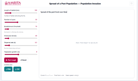
2. The simulator consists of a parameter panel on the left and a graphical visualization panel on the right for displaying the invasion dynamics.

 

3. Specify the habitat length using the Length of habitat (km) slider. This parameter defines the total length of the habitat over which the pest population spreads and determines the number of habitat cells included in the simulation.

 

4. Set the duration of the simulation using the Number of years slider. This parameter specifies the total simulation period over which the spread of the pest population is evaluated.

 

5. Specify the establishment threshold using the corresponding slider. The establishment threshold defines the minimum population density required for a habitat cell to be considered successfully established by the invading pest population.

 

6. Specify the initial pest density using the Initial pest density slider. This parameter determines the initial population density from which the invasion begins.

 

7. Adjust the dispersal rate (d) using the corresponding slider. The dispersal rate represents the fraction of the pest population dispersing to neighbouring habitat cells during each simulation year and determines the rate at which the invasion front advances.

 

8. Set the population growth rate using the corresponding slider. This parameter defines the rate at which the pest population increases within occupied habitat cells between successive simulation intervals.

 

9. After configuring all simulation parameters, click the Plot Graph button to execute the simulation. The simulator computes the spatial spread of the pest population and generates the corresponding graphical output.

 

10. Observe the graph displayed in the visualization panel. The graph illustrates the progression of the pest invasion front over the specified simulation period.

 

11. Interpret the X-axis (Time in years) to determine the duration of the simulation and the Y-axis (Spread Front in km) to examine the distance travelled by the pest invasion front from its initial location.

 

12. Observe the shape and trend of the invasion curve to understand how the pest population spreads through the habitat over time. Compare the spread of the invasion front during the early and later stages of the simulation.

 

13. Use the graph legend to identify the plotted curve representing the spread of the pest front. Move the cursor over the graph, if required, to display the corresponding coordinate values shown beneath the graph. These values indicate the spread distance at a particular simulation year.

 

14. Examine the summary statistics displayed below the graph, including the Final Front and Mean Speed values. These parameters indicate the total distance covered by the invasion front at the end of the simulation and the average rate at which the pest population spreads through the habitat.

 

15. Modify one or more simulation parameters, such as the habitat length, establishment threshold, initial pest density, dispersal rate, population growth rate, or simulation duration, and execute the simulation again to investigate their influence on the progression of the invasion front.

 

16. If required, click the Reset button to restore the default simulation parameters before performing another simulation.

 

17. Download the graphical output by clicking the PNG button or export the numerical simulation data by clicking the CSV button for further analysis and comparison.

 

18. Repeat the above procedure using different parameter combinations to compare invasion rates under varying habitat conditions and identify the factors that accelerate or slow the spread of the pest population.